A Spatiotemporal Hierarchical Bayesian Model for Nonstationary Intensity-Duration-Frequency Curves

James Doss-Gollin

October 13, 2023

Teamwork Makes the Dream Work

Yuchen Lu (Rice)

John Nielsen-Gammon (TAMU)

Rewati Niraula (TWDB)

Benjamin Seiyon Lee (GMU)

Motivation

Today

  1. Motivation

  2. Conceptual Framework

  3. Case study

  4. Ongoing work

  5. Conclusions

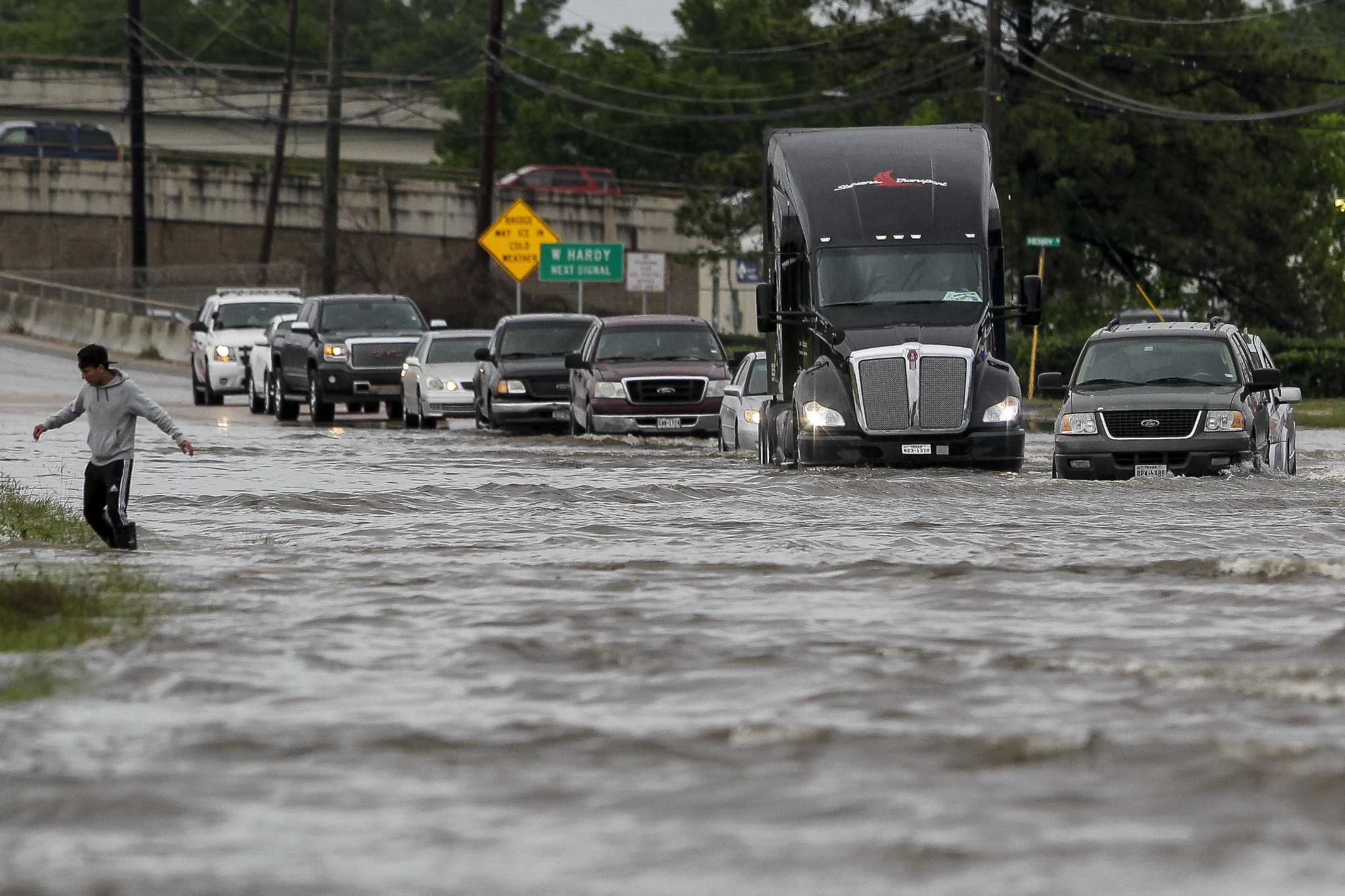
Heavy rainfall: Texas and 🌎

Mesquite, TX, 2022

Houston, 2017

Magnolia, TX, 2016

Houston, 2016

Hong Kong, 2023

Montpelier, VT, 2023

Santa Catarina, Brazil, 2022

Zhengzhou, China, 2021

IDF curves are widely used

Existing guidance leaves gaps

Approach Drawback
Stationarity Accounting for climate change
Point estimate then interpolate Uncertainty quantification / characterization
Separate estimate for each duration Physically inconsistent, high uncertainty
Use gauges w/ long record only Integrate newer gauges (e.g., mesonets)

Key insight

These limitations are most evident at short durations, where the largest changes are anticipated

So what to do?

Conceptual Framework

Today

  1. Motivation

  2. Conceptual Framework

  3. Case study

  4. Ongoing work

  5. Conclusions

Nonstationary extreme value models

Generic nonstationary model for annual maximum precipitation: \[ y(\vb{s}, t) \sim \text{GEV} (\mu(\vb{s}, t), \sigma(\vb{s}, t), \xi(\vb{s}, t)) \]

Process-informed models condition parameters on climate indices \(\vb{X}(t)\) and spatial feature \(\vb{Z}(\vb{s})\) (Cheng & AghaKouchak, 2014; Salas et al., 2018; Schlef et al., 2023) \[ \mu(\vb{s}, t) = \beta(\vb{s}) \times \vb{X}(t) + \alpha \times \vb{Z}(\vb{s}) \]

(optional): same for \(\sigma(\vb{s}, t)\) and \(\xi(\vb{s}, t)\)

Estimation uncertainty

Fagnant et al. (2020)

Serinaldi & Kilsby (2015)

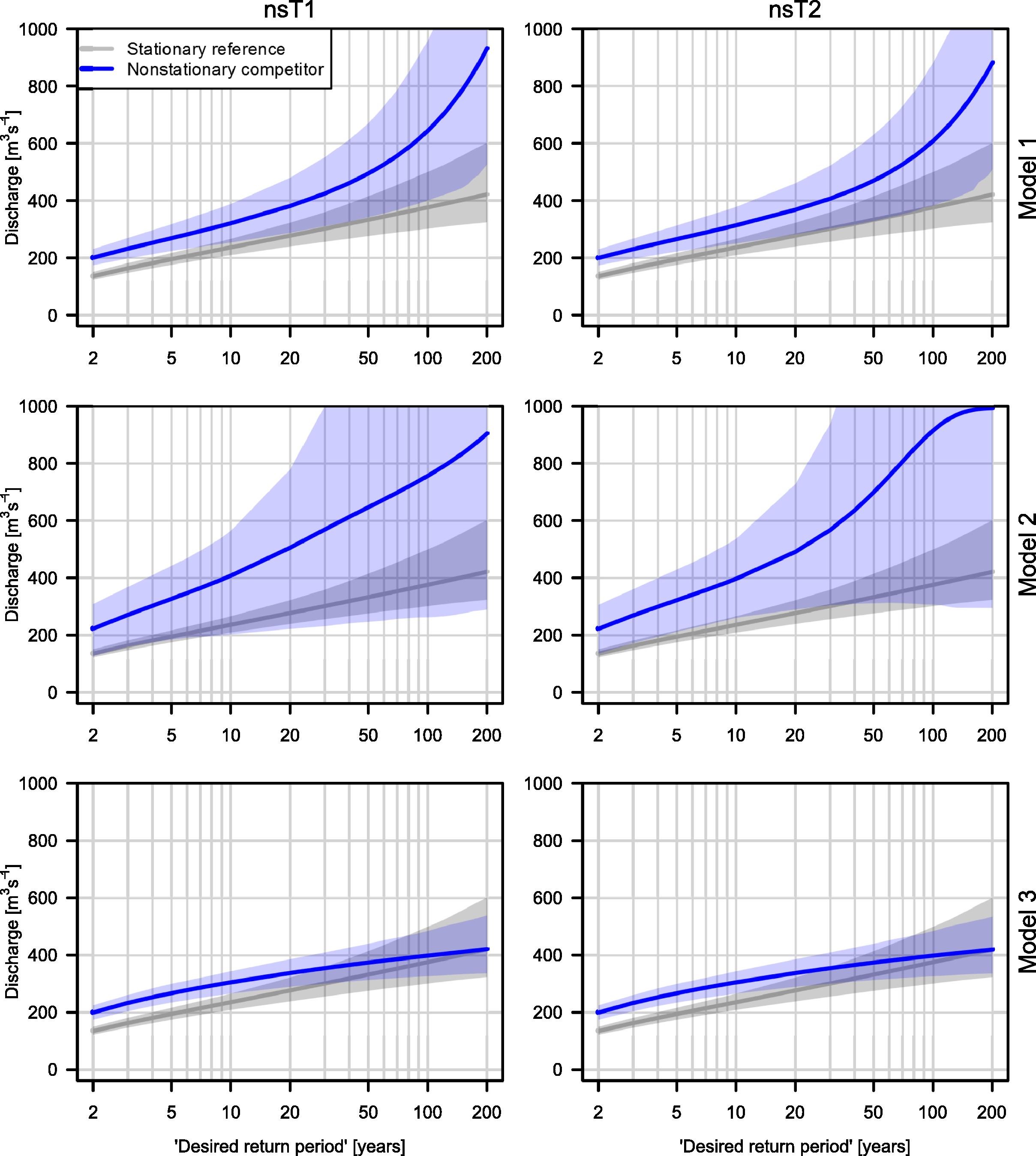
Estimates matter for design & cost

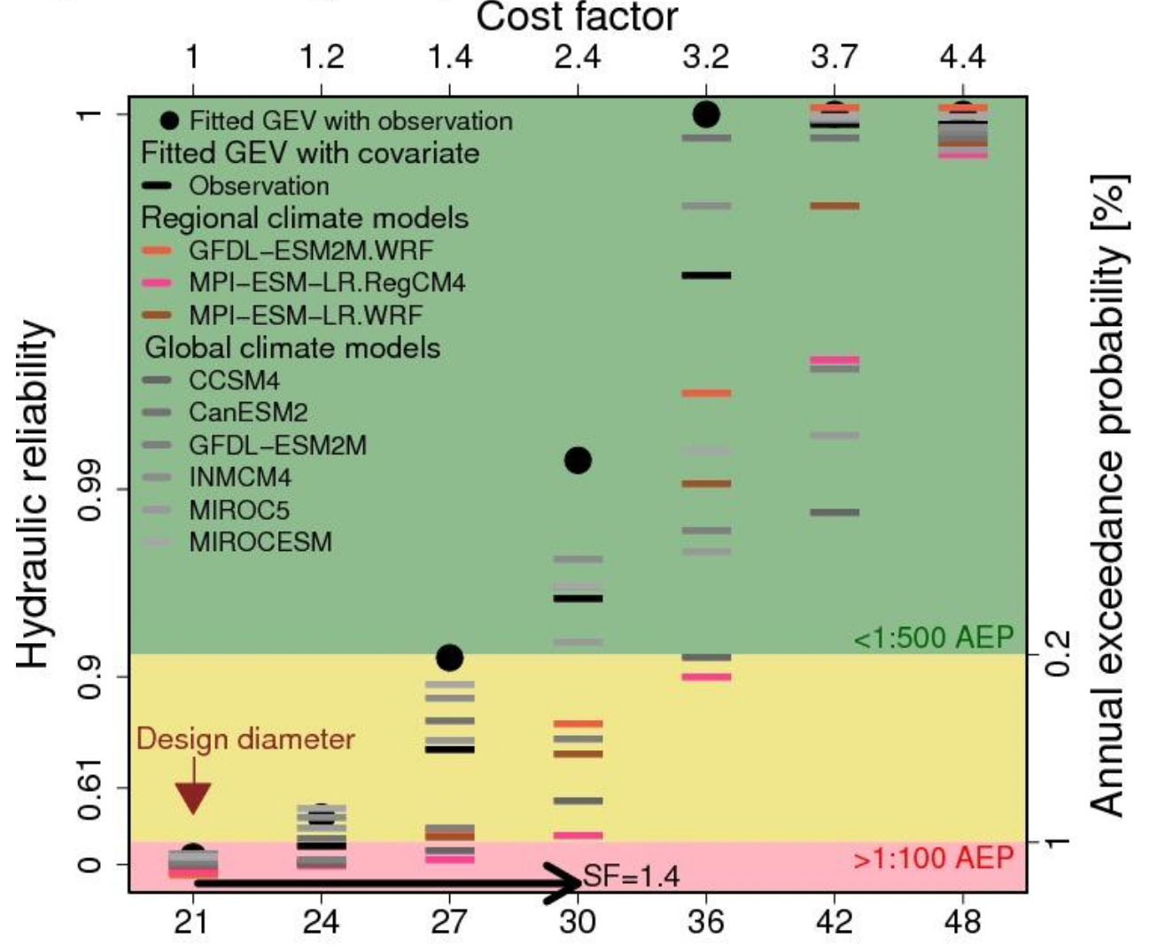
Sharma et al. (2021): Ellicott City, MD

Case study

Today

  1. Motivation

  2. Conceptual Framework

  3. Case study

  4. Ongoing work

  5. Conclusions

Data

Today Ongoing TAMU/TWDB project
NOAA GHCN Extended Atlas-14 and more
Daily Multiple durations
Only stations w/ long record Integrate newer gauges (e.g., mesonets)

Statistical framework

Bayesian hierarichal space-time model (“Spatially Varying Covariates”): \[ \text{Extreme Value Theory} \quad \times \quad \text{Gaussian Processes} \]

  1. Handle varying gauge lengths
  2. Quantify uncertainty in estimates
  3. Assumption: robust effects of climate covariates on the probability distribution of heavy rainfall are heterogeneous in space and time

Flexible inference

We can calculate this map for past, current, or projected global \(\text{CO}_2\) concentrations

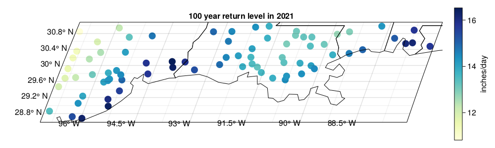
100 year RL for daily precipitation, 2021

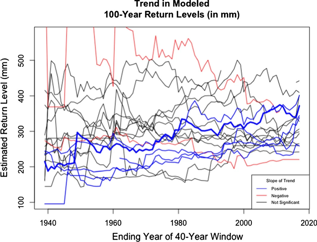
Robust changes in precipitation frequency

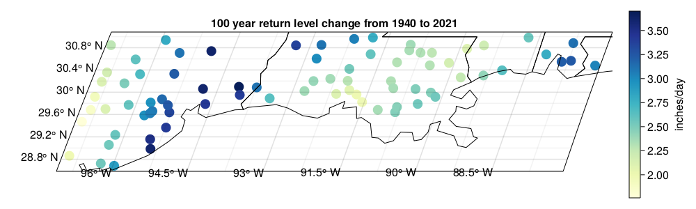
Change in 100 year return level for daily precipitation, 1940-2021

Proabilistic

Fully probabilistic projections at any ungauged location, with uncertainty quantification built-in

Return Plot for Daily Rainfall at Rice University (ungauged, has nearby stations)

Ongoing work

Today

  1. Motivation

  2. Conceptual Framework

  3. Case study

  4. Ongoing work

  5. Conclusions

Parametric duration dependence

Adding a few parameters, we explicitly and flexibly model the GEV parameters as a function of duration \(d\) (Fauer et al., 2021; Koutsoyiannis et al., 1998; Ulrich et al., 2020): \[ \begin{aligned} \sigma (d) &= \sigma_0 (d + \theta) ^ {\eta_1 + \eta_2 } + \tau \\ \mu (d) &= \tilde{\mu} (\sigma_0 (d + \theta ) ^ {-\eta_1 } + \tau) \end{aligned} \]

Fauer et al. (2021)

Integrate climate model simulations

Climate model simulations provide valuable insights, but precipitation is averaged in time and space and represented with substantial biases.

Traditional approaches use climate models directly to

  1. Downscale and bias correct daily/hourly output, then estimate IDF curves
  2. Estimate IDF curves from climate models, then bias correct

Many bias correction pitfalls (see, e.g., Ehret et al., 2012; Lafferty & Sriver, 2023)

We use use climate models indirectly to “play to their strengths”:

  1. Project climate indices
  2. Constrain spatial parameters
  3. Inform duration dependence

Conclusions

Today

  1. Motivation

  2. Conceptual Framework

  3. Case study

  4. Ongoing work

  5. Conclusions

Science to action

Summary

  1. Probabilistic and flexible approach for nonstationary extreme value analysis
  2. Robust estimates
  3. Natural pathway to integrate climate models, duration dependence, and more

dossgollin-lab.github.io

References

Cheng, L., & AghaKouchak, A. (2014). Nonstationary precipitation intensity-duration-frequency curves for infrastructure design in a changing climate. Scientific Reports, 4(1), 7093. https://doi.org/10.1038/srep07093
Ehret, U., Zehe, E., Wulfmeyer, V., Warrach-Sagi, K., & Liebert, J. (2012). Should we apply bias correction to global and regional climate model data? Hydrology and Earth System Sciences, 16(9), 3391–3404. https://doi.org/10.5194/hess-16-3391-2012
Fagnant, C., Gori, A., Sebastian, A., Bedient, P. B., & Ensor, K. B. (2020). Characterizing spatiotemporal trends in extreme precipitation in Southeast Texas. Natural Hazards, 104(2), 1597–1621. https://doi.org/10.1007/s11069-020-04235-x
Fauer, F. S., Ulrich, J., Jurado, O. E., & Rust, H. W. (2021). Flexible and consistent quantile estimation for intensitydurationfrequency curves. Hydrology and Earth System Sciences, 25(12), 6479–6494. https://doi.org/10.5194/hess-25-6479-2021
Koutsoyiannis, D., Kozonis, D., & Manetas, A. (1998). A mathematical framework for studying rainfall intensity-duration-frequency relationships. Journal of Hydrology, 206(1), 118–135. https://doi.org/10.1016/S0022-1694(98)00097-3
Lafferty, D. C., & Sriver, R. L. (2023, April). Downscaling and bias-correction contribute considerable uncertainty to local climate projections in CMIP6. Preprint, Preprints. https://doi.org/10.22541/essoar.168286894.44910061/v1
National Weather Service, & Office of Water Prediction. (2022). Analysis of impact of nonstationary climate on NOAA Atlas 14 estimates.
Salas, J. D., Obeysekera, J., & Vogel, R. M. (2018). Techniques for assessing water infrastructure for nonstationary extreme events: A review. Hydrological Sciences Journal, 63(3), 325–352. https://doi.org/10.1080/02626667.2018.1426858
Schlef, K. E., Kunkel, K. E., Brown, C., Demissie, Y., Lettenmaier, D. P., Wagner, A., et al. (2023). Incorporating non-stationarity from climate change into rainfall frequency and intensity-duration-frequency (IDF) curves. Journal of Hydrology, 616, 128757. https://doi.org/10.1016/j.jhydrol.2022.128757
Serinaldi, F., & Kilsby, C. G. (2015). Stationarity is undead: Uncertainty dominates the distribution of extremes. Advances in Water Resources, 77, 17–36. https://doi.org/10.1016/j.advwatres.2014.12.013
Sharma, S., Lee, B. S., Nicholas, R. E., & Keller, K. (2021). A Safety Factor Approach to Designing Urban Infrastructure for Dynamic Conditions. Earth’s Future, 9(12), e2021EF002118. https://doi.org/10.1029/2021EF002118
Ulrich, J., Jurado, O. E., Peter, M., Scheibel, M., & Rust, H. W. (2020). Estimating IDF Curves Consistently over Durations with Spatial Covariates. Water, 12(11), 3119. https://doi.org/10.3390/w12113119