A Bayesian Spatial Hierarchical Framework for Process-Informed Nonstationary Analysis of Precipitation Frequencies

James Doss-Gollin

Rice University

Yuchen Lu

Rice University

Benjamin Seiyon Lee

George Mason University

November 10, 2023

Teamwork Makes the Dream Work

Yuchen Lu

Benjamin Seiyon Lee

John Nielsen-Gammon

Rewati Niraula

Slides: jdossgollin.github.io/presentations-site

Motivation

Today

1. Motivation

2. Conceptual framework

3. Case study

4. Ongoing work

5. Conclusions

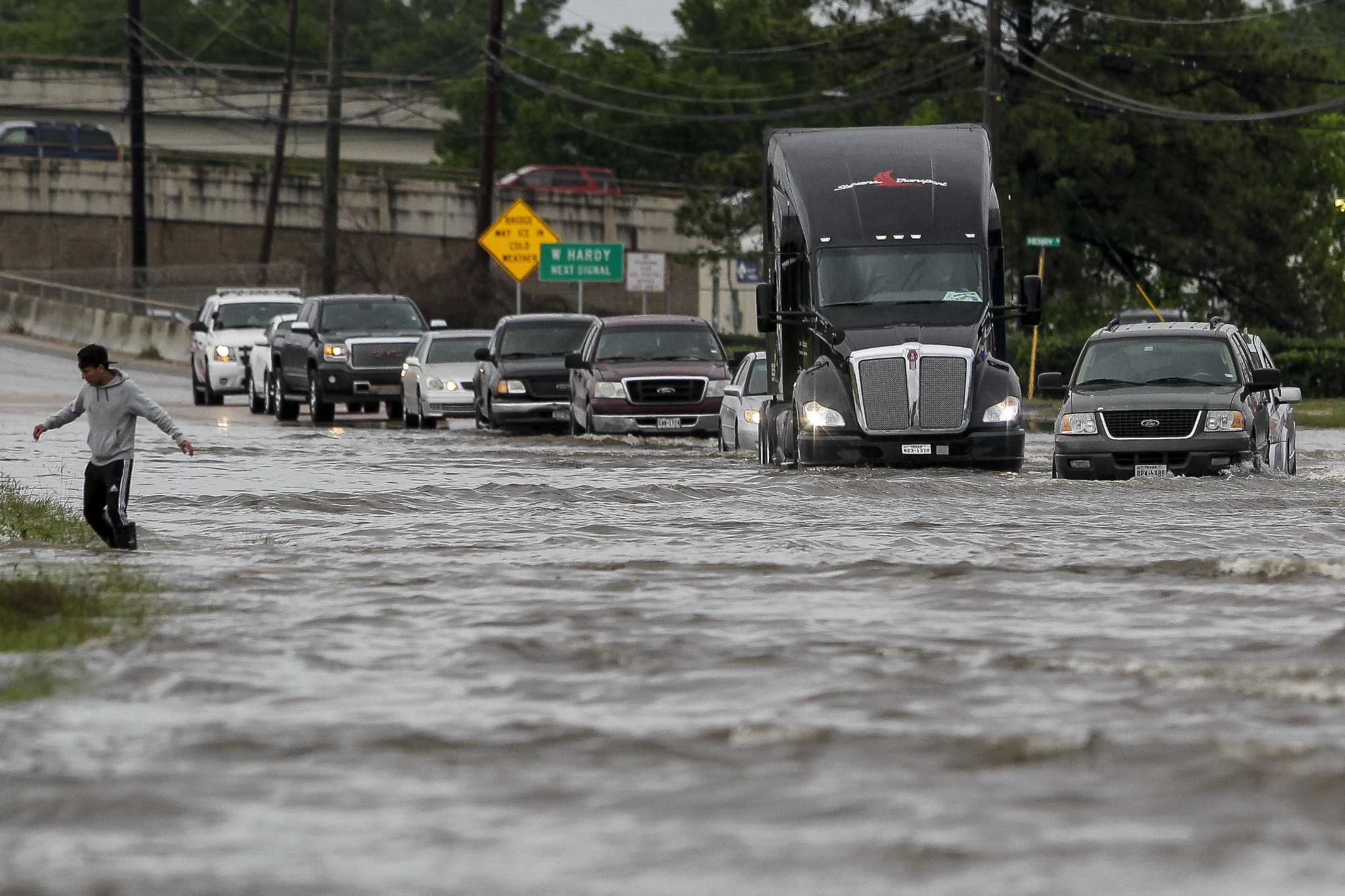
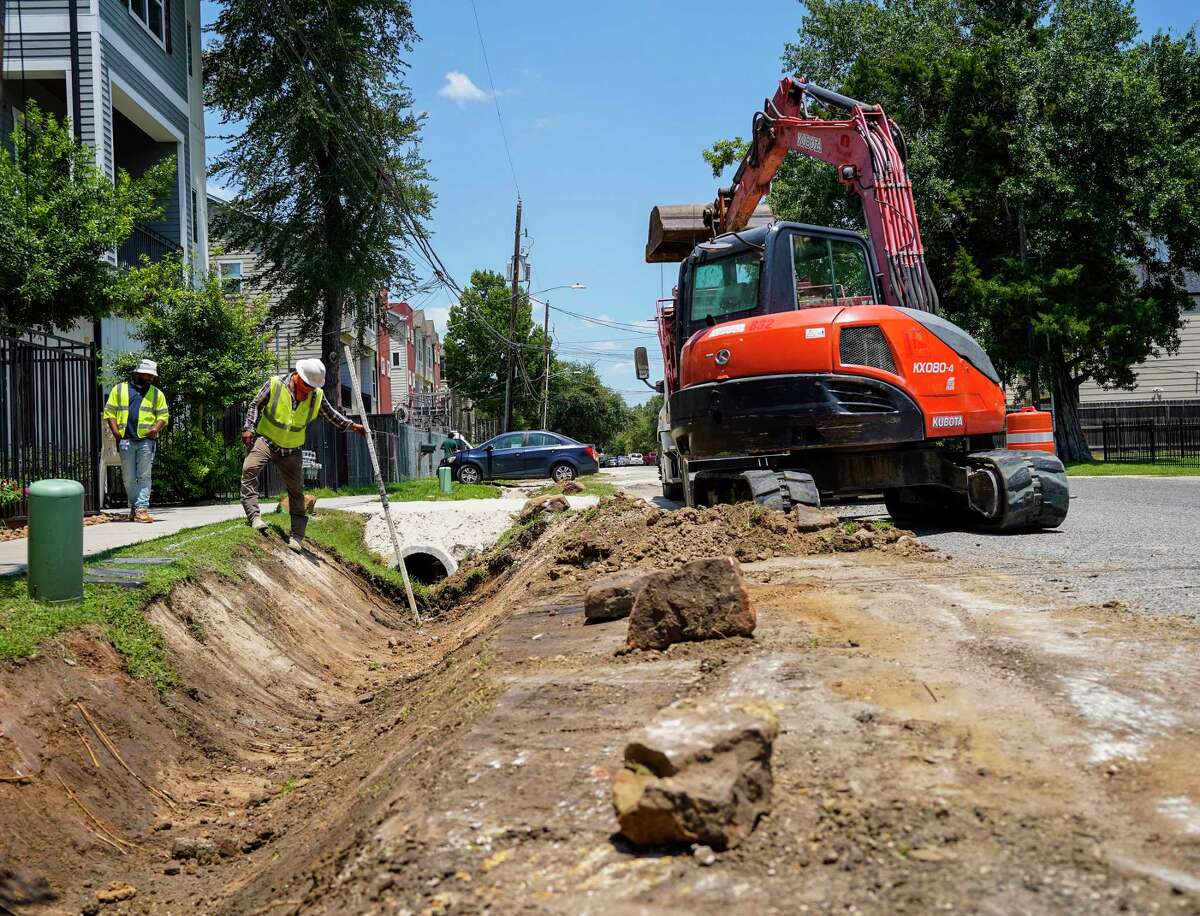
Heavy rainfall: Texas and 🌎

Mesquite, TX, 2022

Houston, 2017

Magnolia, TX, 2016

Houston, TX, 2016

Hong Kong, 2023

Montpelier, VT, 2023

Santa Catarina, Brazil, 2022

Zhengzhou, China, 2021

Figure 1: Engineers use IDF curves for adaptation

Existing guidance leaves gaps

Figure 2: @hydroclim_memes

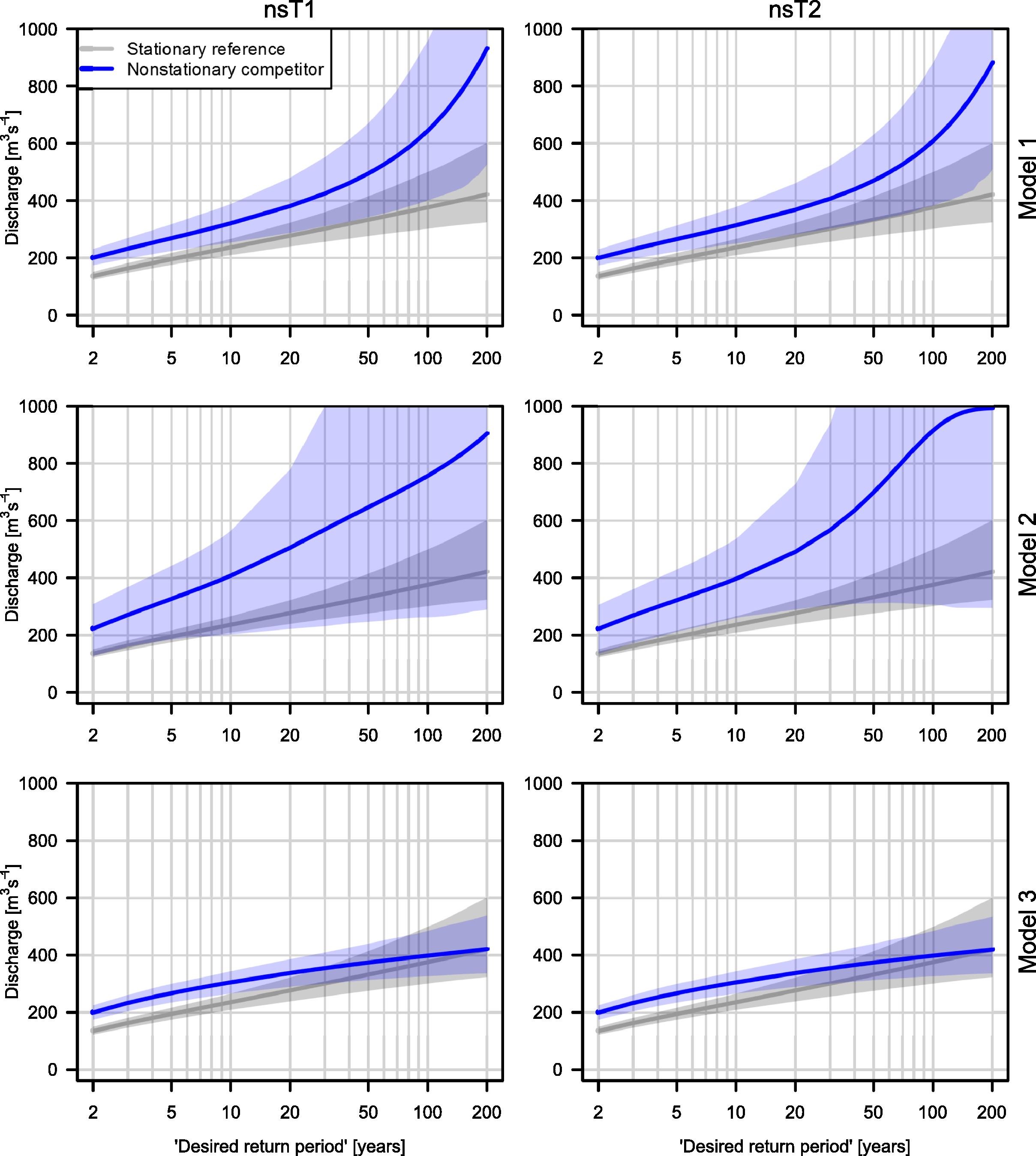
Yet addressing nonstationarity is hard

Figure 3: @hydroclim_memes

Conceptual framework

Today

1. Motivation

2. Conceptual framework

3. Case study

4. Ongoing work

5. Conclusions

Nonstationary extreme value models

Generic nonstationary model for annual maximum precipitation: \[ y(\vb{s}, t) \sim \text{GEV} (\mu(\vb{s}, t), \sigma(\vb{s}, t), \xi(\vb{s}, t)) \]

Process-informed models condition parameters on climate indices \(\vb{X}(t)\) and spatial feature \(\vb{Z}(\vb{s})\) (Cheng & AghaKouchak, 2014; Salas et al., 2018; Schlef et al., 2023) \[ \theta(\vb{s}, t) = \alpha + \beta(\vb{s}) \times \vb{X}(t) + \phi \times \vb{Z}(\vb{s}) \] where \(\theta \in \{\mu, \sigma, \xi \}\)

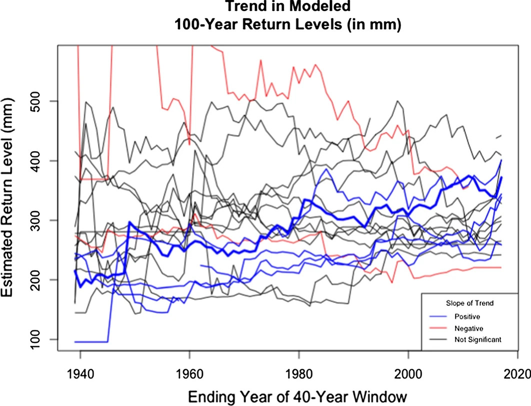
Estimation uncertainty is an Achilles heel

Fagnant et al. (2020)

Serinaldi & Kilsby (2015)

Case study

Today

1. Motivation

2. Conceptual framework

3. Case study

4. Ongoing work

5. Conclusions

Data

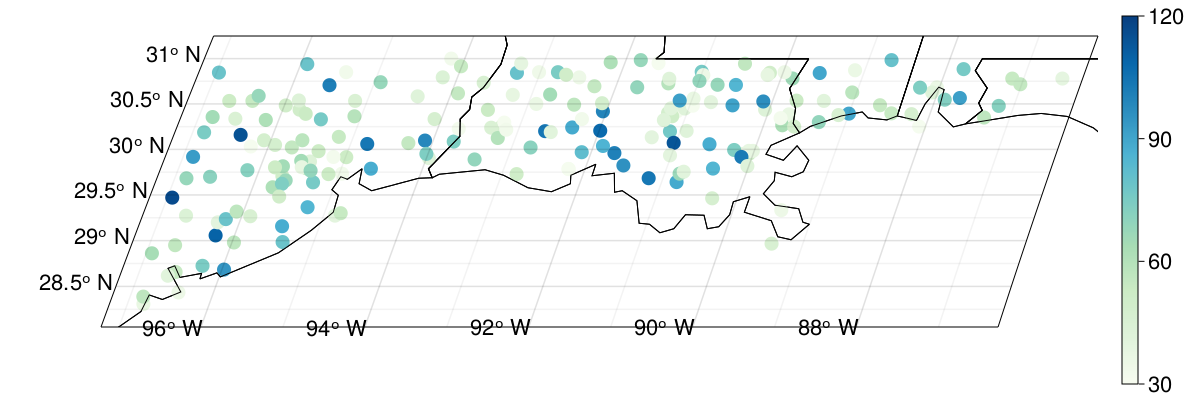
Figure 4: We retain 199 GHCND stations which have at least 30 years with 362+ days of data. Colors indicate number of years of data used.

Spatially Varying Covariates

Bayesian hierarchical space-time model: \[ \begin{aligned} y(\vb{s}, t) &\sim \text{GEV} (\mu(\vb{s}, t), \sigma(\vb{s}, t), \xi) \\ \mu(\vb{s}, t) &= \alpha^\mu + \beta^\mu_1(\vb{s}) \times \ln \text{CO}_2(t) \\ \log \sigma(\vb{s}, t) &= \alpha^\sigma + \beta^\sigma_1(\vb{s}) \times \ln \text{CO}_2(t) \\ \end{aligned} \]

Assume: latent parameters \(\alpha^\mu, \beta^\mu_1, \alpha^\sigma, \beta^\sigma_1\) are smooth in space. Hierarchical spatial prior: \[ \theta(\vb{s}) \sim \text{GP} \left( m, K(\vb{s}, \vb{s}') \right) \] for \(\theta \in \{\alpha^\mu, \beta^\mu_1, \alpha^\sigma, \beta^\sigma_1 \}\) and \(K = \alpha^2 \exp \left(-\frac{ \| \vb{s} - \vb{s}' \| }{\rho} \right)\)

Shifting and widening of the distribution

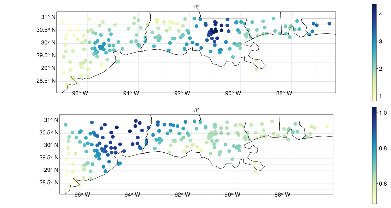
Figure 5: Posterior mean of trend coefficients. Specifically, how much do (T): location parameter and (B): log scale parameter increase with \(\ln \text{CO}_2\)? For reference, an increase from 300 (pre-industrial) to 400 (current) ppm is approximately 0.29 on the log scale and an increase from 400 to 500 (mid-century under RCP 4.5/6) is approximately 0.22.

Estimated return levels}

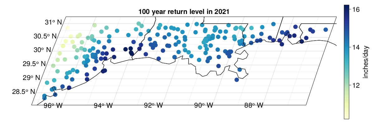
Figure 6: Posterior mean of 100 year return level for 1 day duration at stations, using 2021 covariates (\(\ln \text{CO}_2\)).

Trends and comparison

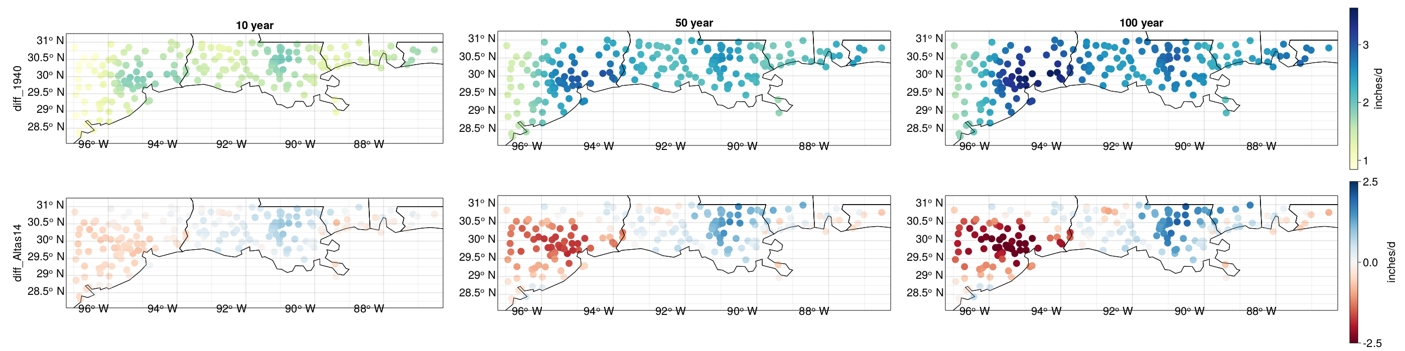
Figure 7: (T): Change in posterior mean of 10, 50, and 100 year return levels from 1940–2021. (B): Difference between our posterior mean for 2021 and Atlas 14. Red (blue) indicates our estimates are lower (higher).

Well-calibrated inferences

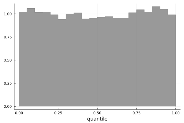
Figure 8: Quantiles of the observation records given the simulated posterior GEV distributions. An ideal model would have a uniform distribution.

Discussion

1. Brand new results – validation ongoing and feedback appreciated
2. Is Atlas 14 too high in SE TX (Nielsen-Gammon, 2020)?
   • Small “region of influence” neglects that Harvey could have hit a wide range
   • Stationary model, short-record stations, sampling only from recent years (Missing at Random)
3. Are our results too low in SE TX?
   • Possible over-smoothing (\(\rho\) large)
   • Daily maxima \(\neq\) 24 hour maxima
   • Separate trends for \(\mu\) and \(\sigma\)

Ongoing work

Today

1. Motivation

2. Conceptual framework

3. Case study

4. Ongoing work

5. Conclusions

More stations (ongoing)

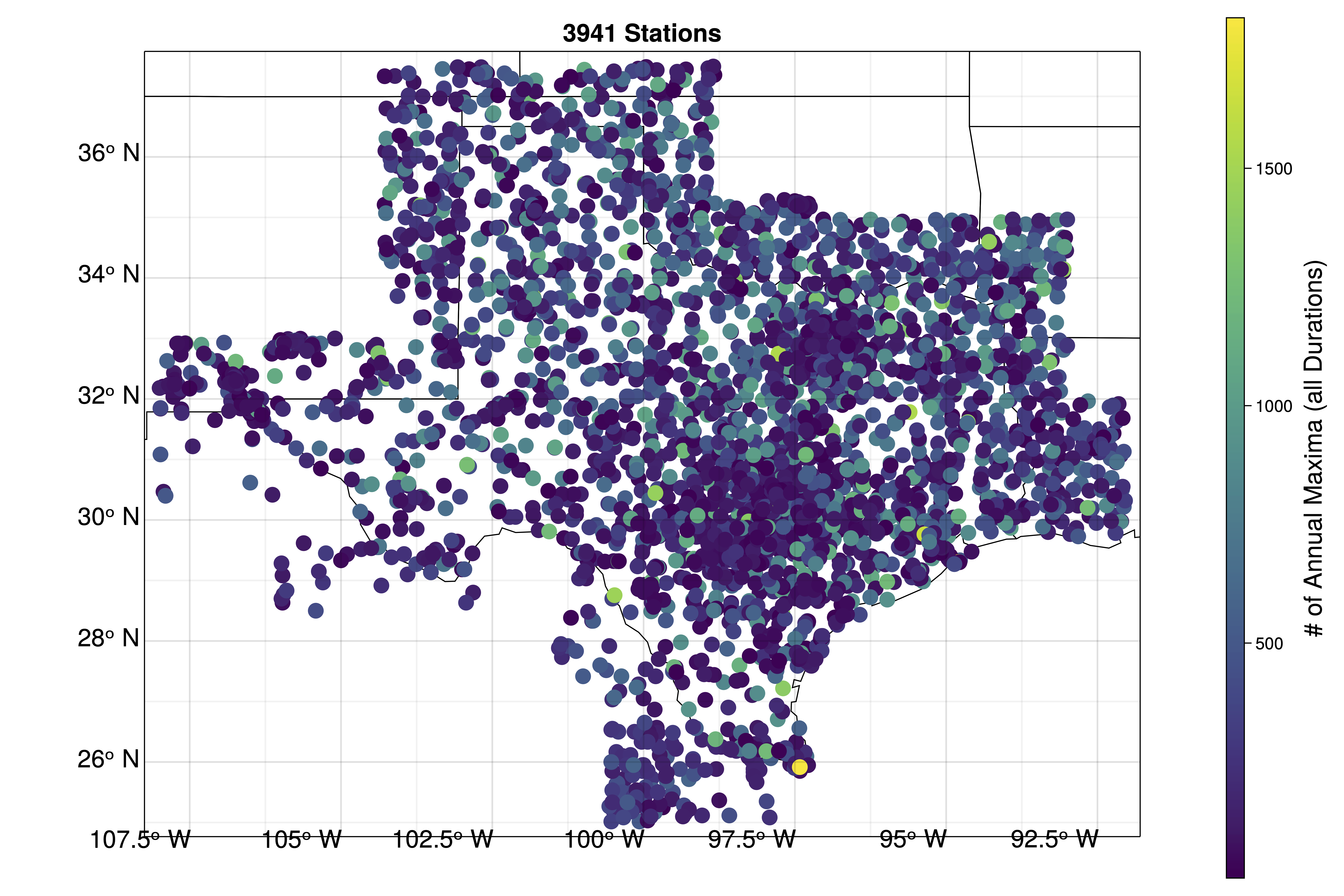
Figure 9: TAMU/TWDB teams have gathered \(>4000\) stations (not all open access). Includes long-duration daily stations, mesonets (short records at high temporal resolution), and more.

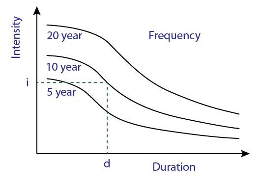
Parametric duration dependence (ongoing)

Adding a few parameters, we explicitly and flexibly model the GEV parameters as a function of duration \(d\) (Fauer et al., 2021; Koutsoyiannis et al., 1998; Ulrich et al., 2020): \[ \begin{aligned} \sigma (d) &= \sigma_0 (d + \theta) ^ {\eta_1 + \eta_2 } + \tau \\ \mu (d) &= \tilde{\mu} (\sigma_0 (d + \theta ) ^ {-\eta_1 } + \tau) \end{aligned} \]

Figure 10: Duration-dependent parameterizations can capture multiple IDF curve behaviors (Fauer et al., 2021)

Conclusions

Today

1. Motivation

2. Conceptual framework

3. Case study

4. Ongoing work

5. Conclusions

Summary

Spatially Varying Covariates Model

1. Bayesian space-time model with latent parameters (including trends) assumed to be smooth in space
2. Flexible approach yields credible inferences
3. Probabilistic framework to integrate future improvements

dossgollin-lab.github.io

References

Cheng, L., & AghaKouchak, A. (2014). Nonstationary precipitation intensity-duration-frequency curves for infrastructure design in a changing climate. Scientific Reports, 4(1), 7093. https://doi.org/10.1038/srep07093

Fagnant, C., Gori, A., Sebastian, A., Bedient, P. B., & Ensor, K. B. (2020). Characterizing spatiotemporal trends in extreme precipitation in Southeast Texas. Natural Hazards, 104(2), 1597–1621. https://doi.org/10.1007/s11069-020-04235-x

Fauer, F. S., Ulrich, J., Jurado, O. E., & Rust, H. W. (2021). Flexible and consistent quantile estimation for intensitydurationfrequency curves. Hydrology and Earth System Sciences, 25(12), 6479–6494. https://doi.org/10.5194/hess-25-6479-2021

Koutsoyiannis, D., Kozonis, D., & Manetas, A. (1998). A mathematical framework for studying rainfall intensity-duration-frequency relationships. Journal of Hydrology, 206(1), 118–135. https://doi.org/10.1016/S0022-1694(98)00097-3

Nielsen-Gammon, J. W. (2020). Observation-based estimates of present-day and future climate change impacts on heavy rainfall in Harris County.

Salas, J. D., Obeysekera, J., & Vogel, R. M. (2018). Techniques for assessing water infrastructure for nonstationary extreme events: A review. Hydrological Sciences Journal, 63(3), 325–352. https://doi.org/10.1080/02626667.2018.1426858

Schlef, K. E., Kunkel, K. E., Brown, C., Demissie, Y., Lettenmaier, D. P., Wagner, A., et al. (2023). Incorporating non-stationarity from climate change into rainfall frequency and intensity-duration-frequency (IDF) curves. Journal of Hydrology, 616, 128757. https://doi.org/10.1016/j.jhydrol.2022.128757

Serinaldi, F., & Kilsby, C. G. (2015). Stationarity is undead: Uncertainty dominates the distribution of extremes. Advances in Water Resources, 77, 17–36. https://doi.org/10.1016/j.advwatres.2014.12.013

Ulrich, J., Jurado, O. E., Peter, M., Scheibel, M., & Rust, H. W. (2020). Estimating IDF Curves Consistently over Durations with Spatial Covariates. Water, 12(11), 3119. https://doi.org/10.3390/w12113119